
Markowitz Modern Portfolio Theory (MPT): How Smart Investors Maximize Profit and Minimize Risk?
When most new investors start, they chase the highest return.
But the world’s best portfolios—managed by hedge funds, banks, and even robo-advisors—do something more intelligent:
✅ They balance return with risk.
✅ They use mathematics to diversify.
✅ They build combinations of assets that grow steadily—even during volatile markets.
This concept is known as Modern Portfolio Theory (MPT), created by economist Harry Markowitz, who later won the 1990 Nobel Prize in Economics.
Why MPT Matters?
MPT proves something powerful:
✅ A portfolio of different assets can be less risky than holding one asset,
even if those individual assets are risky.
This happens because assets do not move exactly the same way at the same time.
Core Concepts of Modern Portfolio Theory
| Idea | Meaning |
|---|---|
| Return | How much an investment earns |
| Risk (Volatility) | How unpredictable the return is |
| Diversification | Mixing different assets to reduce risk |
| Correlation | Measures how assets move together |
1. Correlation & Diversification
Diversification works only if assets do not move in the same direction.
| Correlation Value | Interpretation |
|---|---|
| +1 | Assets move in the same direction (bad diversification) |
| 0 | Assets move independently |
| -1 | Assets move in opposite directions (excellent diversification) |
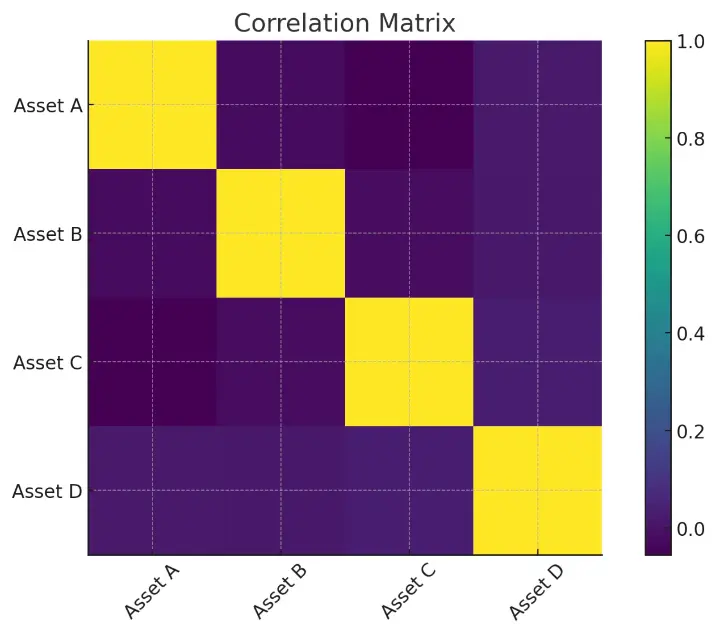
✅ Visualization: Correlation Matrix
import numpy as np
import pandas as pd
import matplotlib.pyplot as plt

np.random.seed(42)

# Generate synthetic returns for 4 assets
returns = np.random.normal(0.001, 0.02, size=(500, 4))
df = pd.DataFrame(returns, columns=['Asset A', 'Asset B', 'Asset C', 'Asset D'])

# Correlation matrix heatmap
corr = df.corr()

plt.figure()
plt.imshow(corr, interpolation='nearest')
plt.xticks(range(len(corr)), corr.columns, rotation=45)
plt.yticks(range(len(corr)), corr.columns)
plt.colorbar()
plt.title('Correlation Matrix')
plt.show()
✅ This heatmap helps visualize which assets move together — and which improve diversification.
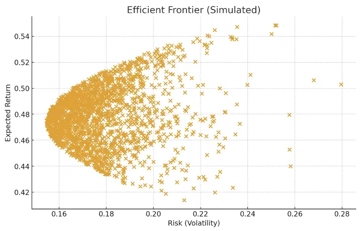
2. Efficient Frontier
The Efficient Frontier shows the best possible portfolios:
✅ Highest return for a given risk
✅ Lowest risk for a given return
Anything below the curve is inefficient — too much risk for too little reward.
✅ Visualization: Simulated Efficient Frontier
weights_list = []
returns_list = []
risk_list = []

for _ in range(2000):
    w = np.random.rand(4)
    w /= np.sum(w)
    weights_list.append(w)
    port_return = np.sum(df.mean() * w) * 252
    port_risk = np.sqrt(np.dot(w.T, np.dot(df.cov() * 252, w)))
    returns_list.append(port_return)
    risk_list.append(port_risk)

plt.figure()
plt.scatter(risk_list, returns_list)
plt.xlabel('Risk (Volatility)')
plt.ylabel('Expected Return')
plt.title('Efficient Frontier (Simulated)')
plt.show()
This scatter plot forms the classic “Markowitz cloud” — showing the risk-return trade-off.
3. Sharpe Ratio & Capital Market Line (CML)
The Sharpe Ratio measures how much return you earn per unit of risk.
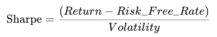
Higher Sharpe = better portfolio.
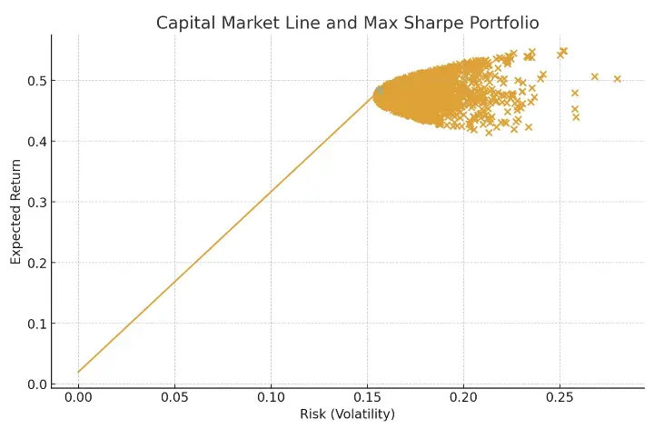
When you mix a risk-free asset (like treasury bills) with your portfolio, you get the Capital Market Line — a straight line that touches the Efficient Frontier at the optimal portfolio (called the tangency portfolio).
✅ Visualization: Capital Market Line + Sharpe Ratio
risk_free_rate = 0.02

# Calculate Sharpe ratios
sharpe_ratios = [(r - risk_free_rate) / s for r, s in zip(returns_list, risk_list)]

# Find portfolio with max Sharpe ratio
max_idx = np.argmax(sharpe_ratios)
max_risk = risk_list[max_idx]
max_return = returns_list[max_idx]

# Capital Market Line
cml_x = np.linspace(0, max_risk, 100)
cml_y = risk_free_rate + sharpe_ratios[max_idx] * cml_x

# Plot Efficient Frontier again + CML
plt.figure()
plt.scatter(risk_list, returns_list)
plt.plot(cml_x, cml_y)
plt.scatter(max_risk, max_return)
plt.xlabel('Risk (Volatility)')
plt.ylabel('Expected Return')
plt.title('Capital Market Line and Max Sharpe Portfolio')
plt.show()
✅ This chart shows:
- the efficient frontier (scatter points),
- the optimal Sharpe portfolio (highlighted point),
- and the Capital Market Line (straight line).
Strengths of Modern Portfolio Theory
✅ Scientifically reduces risk through diversification
✅ Helps avoid emotional investing
✅ Used by banks, funds, and robo-advisors
✅ Creates more stable long-term returns
Limitations of MPT
❌ Assumes markets behave normally
❌ Assumes investors are rational
❌ Correlations change during crises
❌ Extreme market crashes (black swan events) are not well captured
Final Summary
✅ MPT changed how the world invests.
✅ It proves that choosing combinations of assets is smarter than picking just one.
✅ It gives investors a map: maximize reward, minimize risk.
Whether you're investing in stocks, bonds, forex, crypto, or ETFs—MPT provides the scientific foundation for a safer, more profitable portfolio.
Markowitz Modern Portfolio Theory (MPT): Operations Research Behind Smarter Investing